Class 9: Linear Models & Enrichment
Methodology of Scientific Research
Andrés Aravena, PhD
9 Jun 2021
When to use Students’ t
In the cases we see here, we assume that the underlying distribution is Normal
(that is usually the case for averages)
We need to know the population mean and standard deviation
Students’ t when we don’t know population standard deviation
When we have a sample of size 𝑛, we calculate
- sample mean
- sample standard deviation
and we use them to approximate the population values
Then we use Student’s t distribution
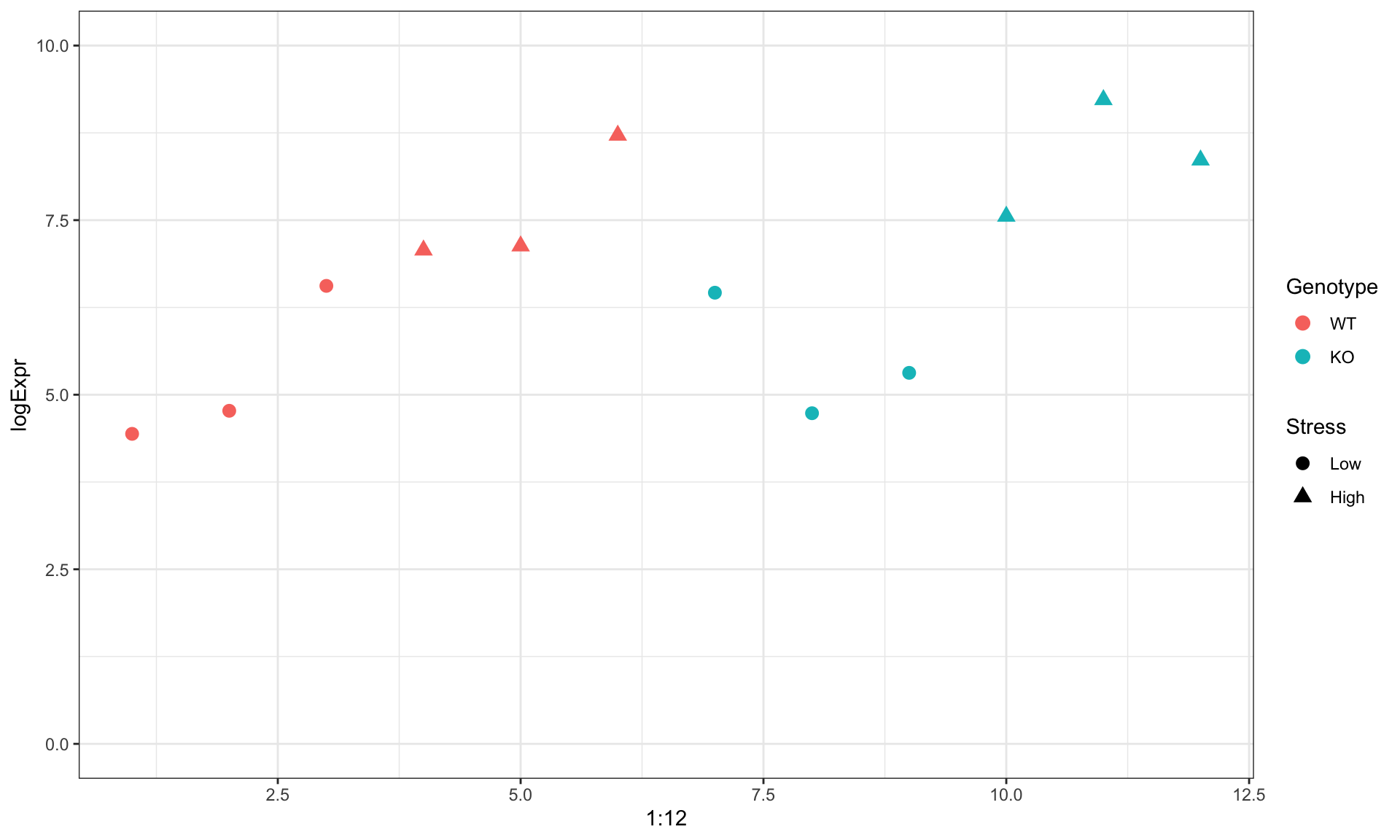
Example: gene expression
| Genotype | Stress | logExpr | |
|---|---|---|---|
| 1 | WT | Low | 4.439524 |
| 2 | WT | Low | 4.769823 |
| 3 | WT | Low | 6.558708 |
| 4 | WT | High | 7.070508 |
| 5 | WT | High | 7.129288 |
| 6 | WT | High | 8.715065 |
| 7 | KO | Low | 6.460916 |
| 8 | KO | Low | 4.734939 |
| 9 | KO | Low | 5.313147 |
| 10 | KO | High | 7.554338 |
| 11 | KO | High | 9.224082 |
| 12 | KO | High | 8.359814 |
Visually
Using a Linear Model
We want to find the change in gene expression due to genotype and stress condition
A common approach is to model gene expression as \[\text{Gene expression} = β_0 + β_1⋅\text{Genotype} + β_2⋅\text{Stress}\]
Here Genotype and Stress are either 0 or 1, depending on the case, and we want to find \(β_0, β_1,\) and \(β_2\) (the coefficients)
Model Matrix
| (Intercept) | GenotypeKO | StressHigh | |
|---|---|---|---|
| 1 | 1 | 0 | 0 |
| 2 | 1 | 0 | 0 |
| 3 | 1 | 0 | 0 |
| 4 | 1 | 0 | 1 |
| 5 | 1 | 0 | 1 |
| 6 | 1 | 0 | 1 |
| 7 | 1 | 1 | 0 |
| 8 | 1 | 1 | 0 |
| 9 | 1 | 1 | 0 |
| 10 | 1 | 1 | 1 |
| 11 | 1 | 1 | 1 |
| 12 | 1 | 1 | 1 |
Fitting the model in R
Most people use the R package limma for gene expression
Here we show a simple version, with one single gene
Call:
lm(formula = logExpr ~ Genotype + Stress)

Coefficients:
(Intercept)   GenotypeKO   StressHigh
     5.1325       0.4941       2.6293
Estimated coefficients are the averages from the sample
Looking at the fitted model
Call:
lm(formula = logExpr ~ Genotype + Stress)

Residuals:
    Min      1Q  Median      3Q     Max
-0.8916 -0.6917 -0.3380  0.8641  1.4262

Coefficients:
            Estimate Std. Error t value Pr(>|t|)
(Intercept)   5.1325     0.4553  11.273 1.31e-06 ***
GenotypeKO    0.4941     0.5257   0.940 0.371872
StressHigh    2.6293     0.5257   5.001 0.000738 ***
---
Signif. codes:  0 '***' 0.001 '**' 0.01 '*' 0.05 '.' 0.1 ' ' 1

Residual standard error: 0.9106 on 9 degrees of freedom
Multiple R-squared:  0.7421,    Adjusted R-squared:  0.6848
F-statistic: 12.95 on 2 and 9 DF,  p-value: 0.002247
Estimated coefficients follow a t distribution
Confidence interval for the coefficients
Estimated coefficients follow a t distribution
We have 12 values, and we evaluate 3 coefficients
Thus, we have 12-3=9 degrees of freedom
Then we can use the 9 DF table of Student’s t to get a confidence interval
                 2.5 %   97.5 %
(Intercept)  4.1025560 6.162410
GenotypeKO  -0.6952039 1.683310
StressHigh   1.4400824 3.818597
Interpretation
                 2.5 %   97.5 %
(Intercept)  4.1025560 6.162410
GenotypeKO  -0.6952039 1.683310
StressHigh   1.4400824 3.818597
(Intercept) is the base expression level for Wild Type and Low Stress
GenotypeKO is the differential expression due to gene KO. It can be 0, so we do not have enough evidence to say “there is an effect”
StressHigh is the differential expression due to stress. It seems greater than 0 at 95% confidence. Will still be >0 at 99% confidence?
𝑝-values
Call:
lm(formula = logExpr ~ Genotype + Stress)

Residuals:
    Min      1Q  Median      3Q     Max
-0.8916 -0.6917 -0.3380  0.8641  1.4262

Coefficients:
            Estimate Std. Error t value Pr(>|t|)
(Intercept)   5.1325     0.4553  11.273 1.31e-06 ***
GenotypeKO    0.4941     0.5257   0.940 0.371872
StressHigh    2.6293     0.5257   5.001 0.000738 ***
---
Signif. codes:  0 '***' 0.001 '**' 0.01 '*' 0.05 '.' 0.1 ' ' 1

Residual standard error: 0.9106 on 9 degrees of freedom
Multiple R-squared:  0.7421,    Adjusted R-squared:  0.6848
F-statistic: 12.95 on 2 and 9 DF,  p-value: 0.002247
Expression v/s Fold Change

Volcano plot

Doing Multiple tests
The problem with multiple tests

Multiple test correction
There are several approaches
- Family Wise Error Rate control (Bonferroni)
- False Discovery Rate control (Hochberg)
- Others
The basic difference is the trade-off between False Positives and False Negatives
Two ways of being wrong
In every hypothesis test, we can be wrong in two ways
- Type 1: False positive
- putting innocents in the jail
- Type 2: False negatives
- freeing criminals
Usually improving one means worsening of the other
How does FWER work
Family Wise Error Rate multiplies each p-value by the number of cases \[p.adj = p.value ⋅ N\]
It reduces False Positives and increases False Negatives
Sometimes we get nothing significant
How does FDR work
FDR sorts the p-values and multiplies each by an increasing value \[\text{p.adj} = \text{p-value} \cdot\frac{i}{N}\]
If we get \(p.adj<0.05\) then the probability that it is a false positive is 5%
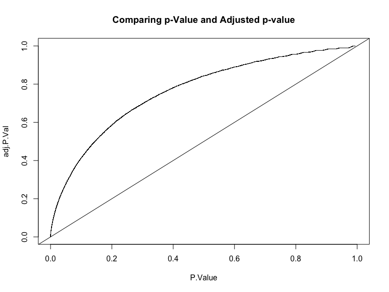
Original v/s adjusted p-value
Looking for Biological meaning
Enrichment analysis
At this point we have a list of DE genes
Let’s say they are 10% of all genes
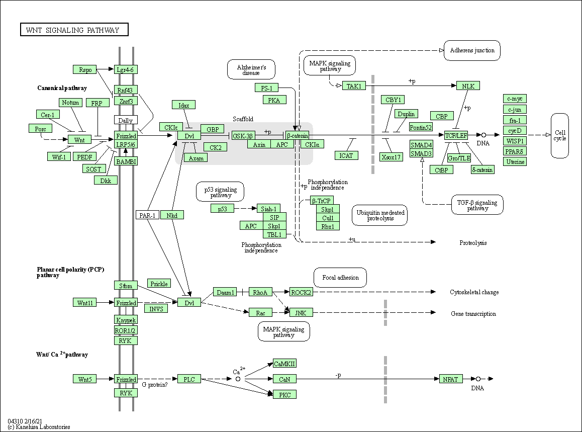
Each gene is part of one or more networks
- Enzimes are in metabolic networks
- Transcription factors are in regulatory networks
- and regulated genes also
- Other genes are part of signaling networks
We can draw expression on a network
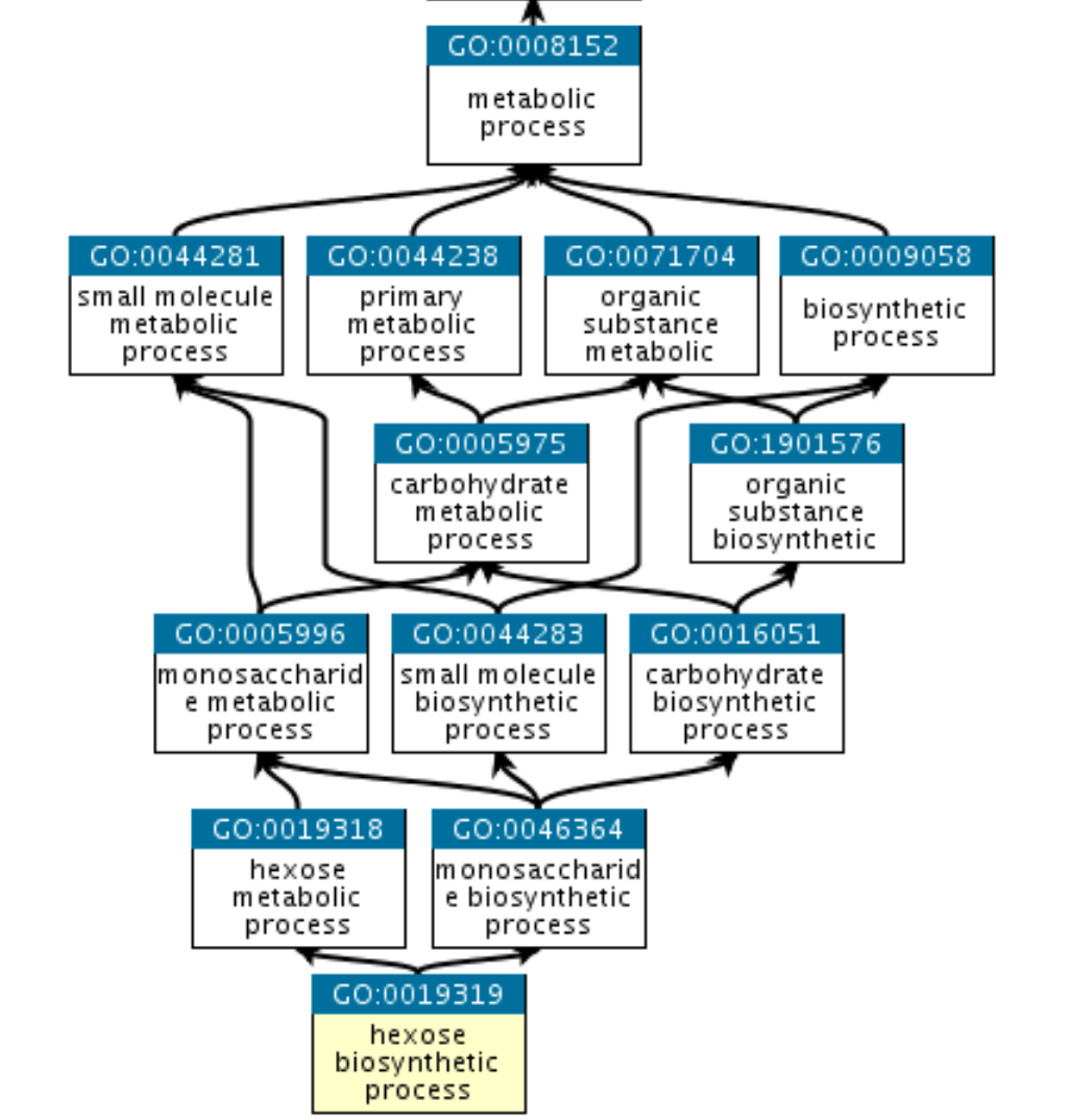
Gene Ontology
Beyond pathways, it is useful to look at “Gene Ontology”
It has three branches
- Molecular Function
- Cellular Component
- Biological Process
GO is a graph
Which networks shall we look at?
To find the relevant networks, we use Enrichment Analysis
For example, let’s say we have 10000 genes in total, and 1000 DE genes
Let’s say that carbon metabolism takes 3000 genes in total
If, among the DE genes, 300 genes are in carbon metabolism, we will not be surprised
Is this random or not?
3K carbon metabolism in 10K total genes is 30%
If we take 1K random genes, we expect to have 30% of them in carbon metabolism, just by randomness
If instead we have 600 carbon metabolism among the 1K DE genes, we are surprised
In that case we say that the set of carbon metabolism is enriched in the DE experiment
How to do enrichment analysis
This problems follows an hypergeometric distribution
\[ℙ(k \text{ observed sucesses} | N,K,n)\]
- \(N\) is the population size,
- \(K\) is the number of success states in the population
- \(n\) is the number of draws (i.e. quantity drawn in each trial)
- \(k\) is the number of observed successes
In our terms
\[ℙ(k \text{ DE genes in group} | N,K,n)\]
- \(N\) is the total number of genes,
- \(K\) is the total number of genes in the group
- \(n\) is the number of DE genes
- \(k\) is the number of DE genes in the group