Class 13: Systems of linear equations
Systems Biology
Andrés Aravena, PhD
December 28, 2023
Normal distibution
\(X\) follows a Normal(0,1) iff
\[ℙ(X>a) = \frac{1}{K} \int_{-\infty}^a e^{-\frac{1}{2} x^2} dx\]
Here \(K\) is chosen so total probability is 1
\[K = \int_{-\infty}^\infty e^{-\frac{1}{2} x^2} dx=\sqrt{2\pi}\]
Two independent variables
\[ \begin{aligned} ℙ(X_1>t_1, X_2>t_2) &= ℙ(X_1>t_1) ℙ(X_2>t_2)\\ &= \left(\frac{1}{K} \int_{-\infty}^{t_1} e^{-\frac{1}{2} x_1^2} dx_1\right) \left(\frac{1}{K} \int_{-\infty}^{t_2} e^{-\frac{1}{2} x_2^2} dx_2\right)\\ &= \frac{1}{K^2} \int_{-\infty}^{t_1} \int_{-\infty}^{t_2} e^{-\frac{1}{2} x_1^2} e^{-\frac{1}{2} x_2^2} dx_2 dx_1\\ &= \frac{1}{K^2} \int_{-\infty}^{t_1} \int_{-\infty}^{t_2} e^{-\frac{1}{2} (x_1^2+x_2^2)} dx_2 dx_1\\ &= \frac{1}{K^2} \int_{-\infty}^{t_1} \int_{-\infty}^{t_2} e^{-\frac{1}{2} 𝐱^T𝐱} dx_2 dx_1\\ \end{aligned} \]
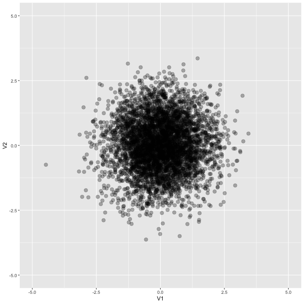
Graphic

Changing scale
Let \(U_1 = a⋅X_1\) and \(U_2 = d⋅X_2\). What is \(ℙ(U_1, U_2)\)?
Since we have \(X_1 = U_1/a\) and \(X_2 = U_2/d\), we get
\[ ℙ(U_1, U_2) = \frac{1}{K^2} \int\int \exp\left(-\frac{1}{2} (\frac{u_1^2}{a^2}+ \frac{u_2^2}{d^2})\right) \frac{du_1}{a}\,\frac{du_2}{d} \]
We can write
\[ \frac{u_1^2}{a}+\frac{u_2^2}{d} = 𝐮^T\begin{bmatrix} 1/a^2 & 0\\ 0 & 1/d^2\end{bmatrix}𝐮= 𝐮^T\begin{bmatrix} a^2 & 0\\ 0 & d^2\end{bmatrix}^{-1}𝐮 \]
Combinig variables
Let \(U_1 = a⋅X_1 + b⋅X_2\) and
\(U_2 = c⋅X_1+d⋅X_2\).
That is
\[ \begin{bmatrix} U_1\\U_2\end{bmatrix} = \begin{bmatrix}a&b\\c&d\end{bmatrix} \begin{bmatrix}X_1\\X_2\end{bmatrix} \]
which we can write as \(𝐮=A𝐱\). Thus \(𝐱=A^{-1}𝐮\)
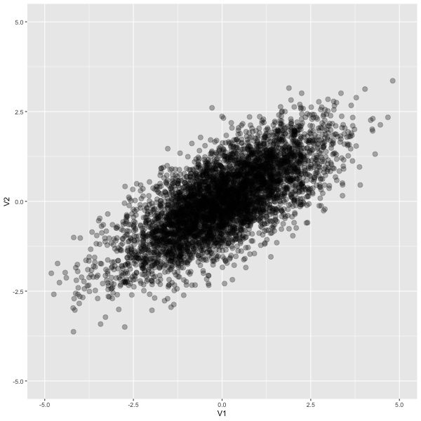
It looks like this

New probability
\[\frac{1}{K^2} \int\int \exp\left(-\frac{1}{2}(A^{-1}𝐮)^T A^{-1}𝐮\right)\det(A^{-1}) du_1\,du_2\] \[\frac{1}{K^2}\det(A^{-1}) \int\int \exp\left(-\frac{1}{2}𝐮^T (A^{-1})^T A^{-1}𝐮\right) du_1\,du_2\]
Determinant
How to calculate 𝐾
Detereminant of product
\[\det(AB)=\det(A)\det(B)\] \[\det(AI)=\det(A) ⇒ \det(I)=1\]
\[\det(A^{-1})=\det(A)^{-1}\]
Trace
Trace of a product
probability again
\[\frac{1}{K^2 \det(A)} \int\int \exp\left(-\frac{1}{2}𝐮^TA^{-T} A^{-1}𝐮\right) du_1\,du_2\] where \(A^{-T}\) is short for \((A^{-1})^T\). Notice that \[(A^{-T} A^{-1})(AA^T)=A^{-T} (A^{-1}A)A^T=A^{-T}A^T=I\] thus \(A^{-T} A^{-1}=(AA^T)^{-1}\)
Naming the new matrix
We will write \(AA^T=Σ\) and then we have \[\det(\Sigma)=\det(A)\det(A^T) = \det(A)^2\] then the probability is
\[ \frac{1}{K^2\det(\Sigma)^{-1/2}} \int\int \exp\left(-\frac{1}{2}𝐮^T\Sigma^{-1}𝐮\right) du_1\,du_2 \]
For more than 2 variables
If we have \(m\) variables (maybe genes) then \(ℙ(U_1,…, U_m)\) is
\[ \frac{1}{K^m\det(\Sigma)^{1/2}} \int\int \exp\left(-\frac{1}{2}𝐮^T\Sigma^{-1}𝐮\right) du_1\ldots du_m \]
\[ \frac{1}{\sqrt{(2\pi)^m\det(\Sigma)}} \int\int \exp\left(-\frac{1}{2}𝐮^T\Sigma^{-1}𝐮\right) du_1\ldots du_m \]
Interpretation
The key part here is \[𝐮^T\Sigma^{-1}𝐮\] This means that the relationship between variables is contained in the matrix \(Θ=Σ^{-1}\)
\(Θ\) is called precision matrix
\(Σ\) is called covariance matrix
So we just need to find the inverse of the covariance
We cannot do that
What we can do instead
Maximum likelihood
Taking logs
divide by \(-n\) (Now we minimize)
\[S=\frac{1}{n}X^T X\]
What we look for
\[\min_\Theta \left(\text{tr}(S\Theta)-\log\det(\Theta)\right)\]